V. Microscopy
This section contains a lot of material.
Sections A and B, written in the first person, discuss how to grow and observe Clarkia pollen.
Section C contains observations and analysis of of amyloplast and spherosome sizes and Brownian motion.
There is a digression to discuss the effect of a lens on observed spherosome sizes, so that the real size may be inferred from the observed size.
The section concludes with instructions how to construct a ball lens microscope, and discussion of some observations of amyloplast sizes made with it.
A. Growing Clarkia
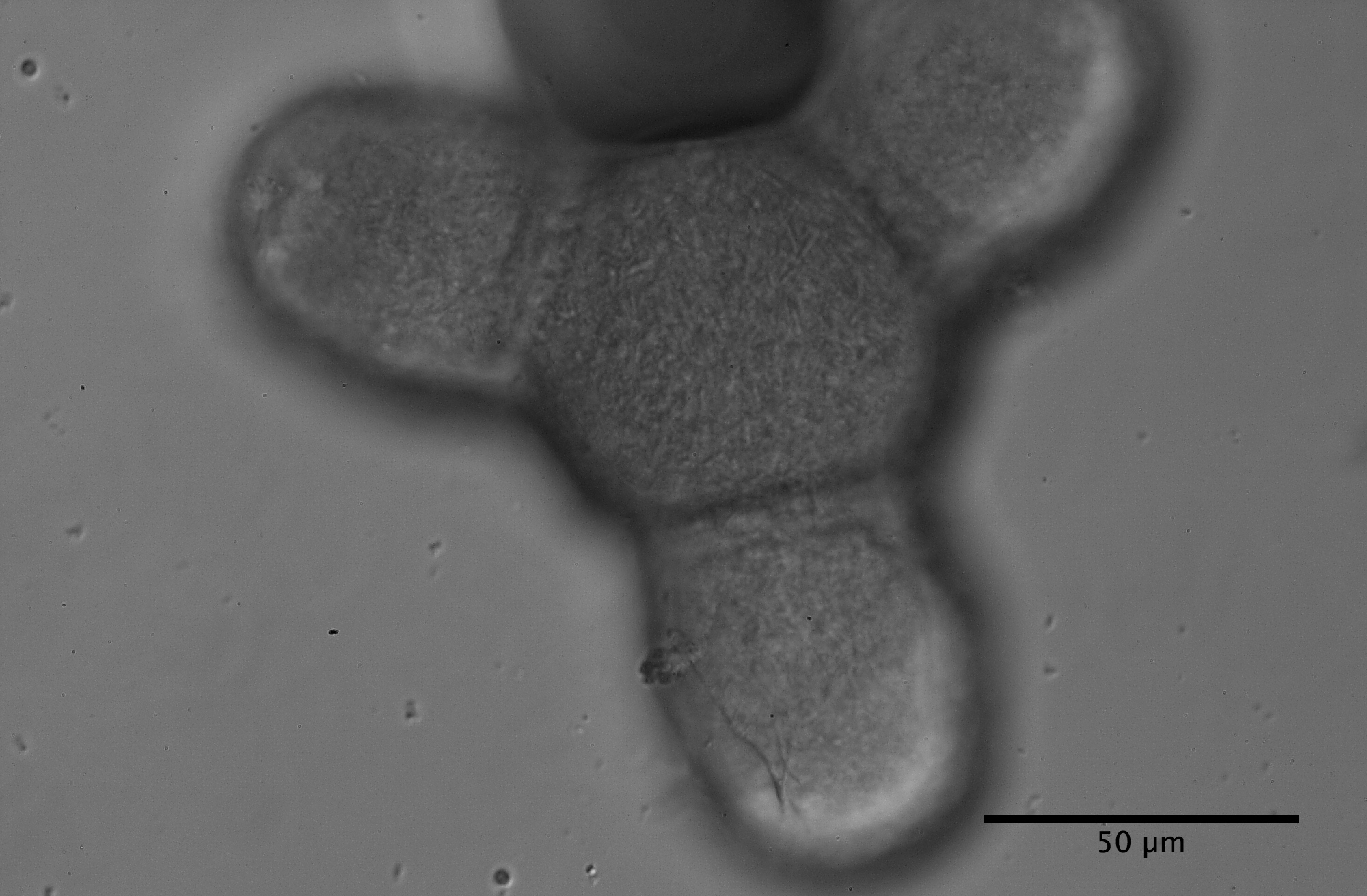
Clarkia pulchella, variously called ragged robin, elkhorn, pinkfairies and deerhorn (because of its four three-pronged petals), is native to western North America. It can be found growing wild in parts of British Columbia, Idaho, Montana, South Dakota and Washington.(1)
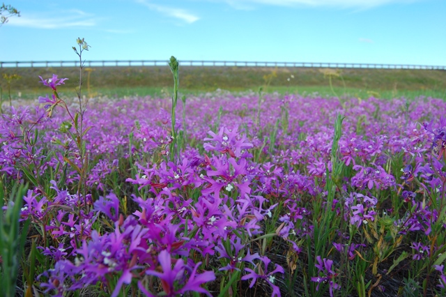 |
| Field of Clarkia pulchella |
Indeed, I observed some sent to me that grew wild near Missoula, Montana. However, a number of companies sell Clarkia pulchella seeds,(2) along with seeds of Clarkia amoena (also called farewell-to-spring), which grows wild in California, Oregon and Washington, and seeds of Clarkia elegans (also called unguiculata, mountain garland) which grows wild in California. Seed packets sell for just a few dollars. (Other Clarkia species, of which 41 are known,(3) are sold less frequently).
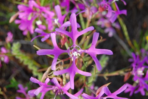 |
| Clarkia pulchella flowers |
Seed--growing advice is available on--line and in many gardening books. Growing seeds indoors under lights is not hard. Here is one person's experience, which certainly can be improved upon. My aim was to do as little as possible.
There are many seed growing systems available at gardening stores, such
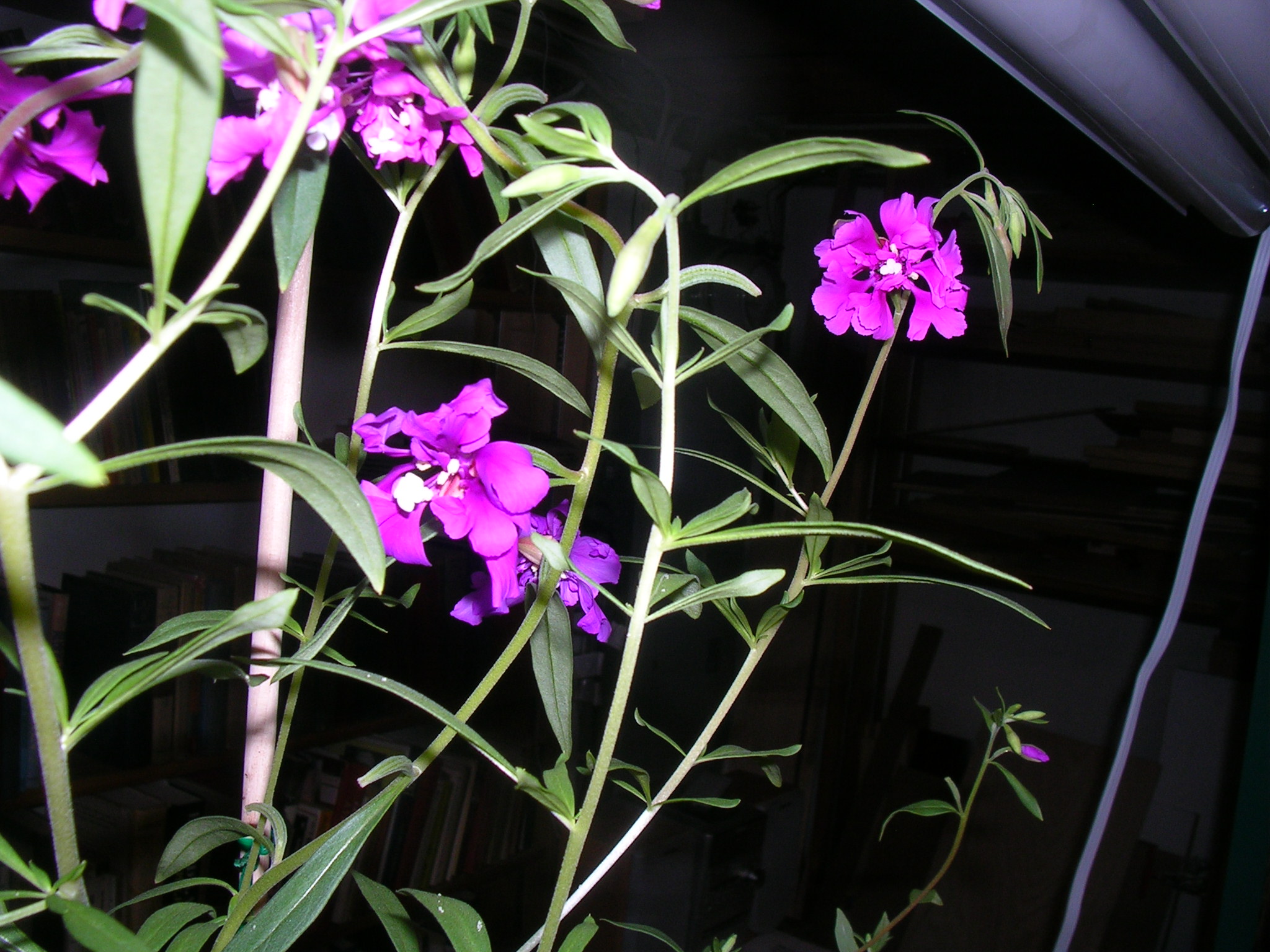 |
| Clarkia pulchella growing in my basement |
as peat pots. I have had good results with the Lee Valley Self-Watering Seed Starter,(4) which contains 24 compartments, watering via a felt capillary mat, and a water level indicator. It can be left for about a week before refilling with water. The mat should be soaked before using. Lee Valley recommends using a soil-less mixture containing sphagnum or peat, but I used a commercial potting soil mix with added nutrients.
 |
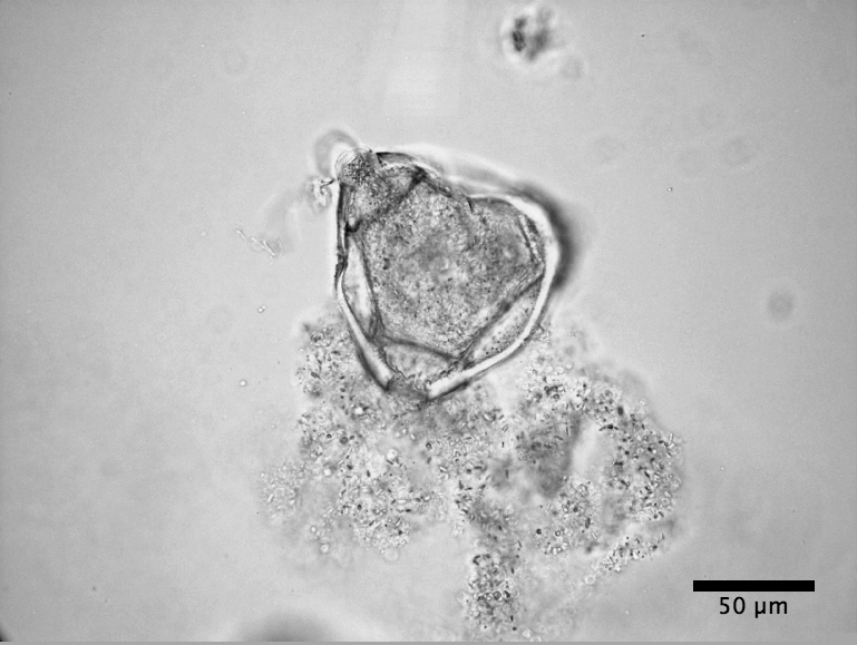
| Clarkia pulchella pollen imaged under a microscope at x400. |
A shop light fixture with grow--light bulbs, or even ordinary fluorescent bulbs, can be used, with some arrangement to raise the plants or lower the light fixture. However, I used a commercial stand with grow--lights which is reasonably priced(5) and has a mechanism for raising and lowering the fixture. A timer that kept the lights on perhaps 16 hours a day completed the equipment.
Seeds may be meted out to the compartments from the seam of
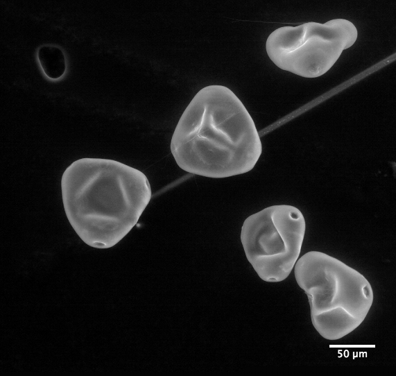 |
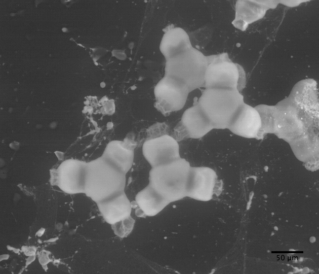
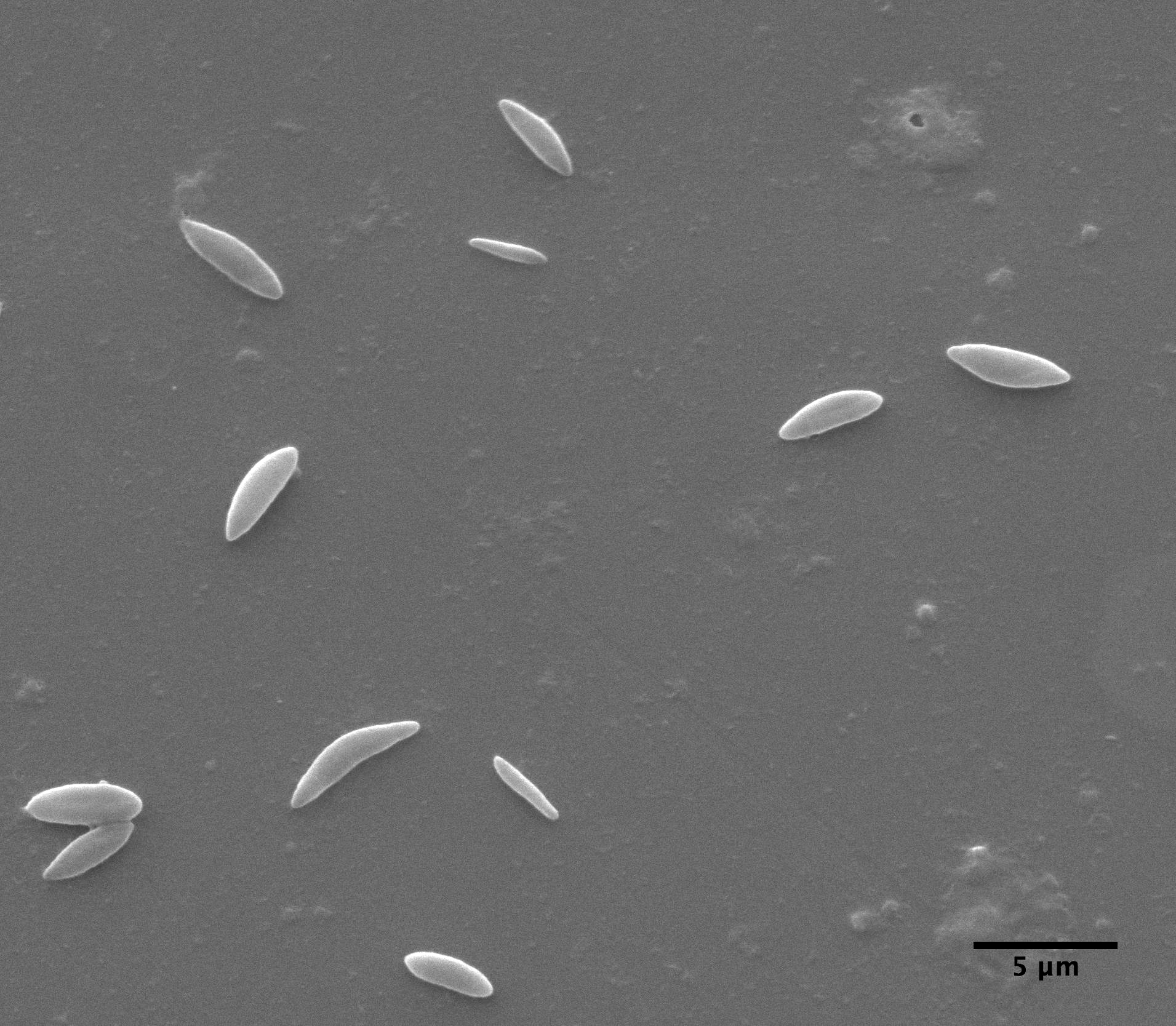
| Clarkia pulchella imaged by an electron microscope |
a small folded piece of paper. The seeds germinated in about a week to ten days. The bulbs should be within a few inches of the tops of the plants, else theplants become etoliated, i.e., spindly from lack of sufficient light. After a few weeks to a month, I transferred the seedlings to 4" pots, 24 of which fit in a tray (periodically watered).(4) As the plants grew, I staked them. Flowers started to bloom after about ten weeks.
B. Qualitative
 |
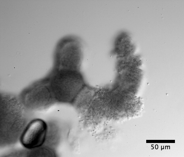
| Clarkia Pulchella pollen bursting (see video) |
C. pulchella has four stamens surrounding the pistil. I used a miniature Swiss army knife scissors (a nail scissors will do as well) to cut each filament so the anther fell on a microscope slide. I used tweezers to hold an anther. If the anther had not yet burst, I sliced it with a long sharp sewing needle to reveal the pollen. If it had burst, usually some pollen had fallen out of the anther and was already on the slide. In either case, I scraped pollen out of the anther with the needle. I enjoyed observing what I was doing through a low power binocular microscope, though this can be done without one. C. pulchella pollen are little triangles, which glowed in the light like diamonds.
 |
| Clarkia amoena pollen under the microscope x400 |
I was surprised when I did the same with C. amoena and C. elegans. I had not known that species of the same genus could have differently shaped pollen, in this case hexagons with protuberant lobes on alternate edges. The connection between the two shapes is apparent when viewing a dry slide of desiccated C. pulchella pollen. Each appears as a membrane surrounding the C. amoena/C. elegans pollen shape (see below).
A drop of distilled water is put on the pollen on the slide using a medicine dropper, followed by a cover slip and then observed. One should follow
 |
| Clarkia elegans pollen under the electron microscope |
Brown's injunction to observe pollen from anthers either before dehiscence (i.e., before the anther has split open, releasing the pollen) or soon thereafter. Most of the pollen do not burst in water, and if one waits too many days after dehiscence to make observations, none may burst, especially for Clarkia pulchella. As pollen matures in the anther, its outer membrane may grow more impervious to bursting in water.
When first viewed, particles from the pollen were sometimes seen already on the slide: perhaps the pollen hadbeen damaged by the needle, or the pollen had rapidly burst open as soon as the water was applied. I could also see pollen bursting before my eyes (see videos), and the particles streaming out like logs released from a log--jam, usually in fits and starts. The particles at the log-jam perpihery
 |
| Clarkia elegans pollen bursting (see video) |
diffuse away from the rest and can be seen undergoing Brownian motion. The remainder are packed closely, and the intracellular medium in which they sit is viscous, so they show little or no Brownian motion until the log--jam disperses.
C. Quantitative
There are many interesting phenomena one can investigate. Here are two brief studies, suggestive but by no means definitive. For the first, we
 |
| Dessicated Clarkia pulchella pollen |
consider the distribution of particle sizes emerging from Clarkia pulchella pollen before and after dehiscence. For the second, we consider Brownian motion and Brownian rotation of the amyloplasts.
C1.Observations
An Olympus BX-50 microscope, at x400 was used. Its resolution is cited as .45 microns, and its depth of focus as 2.5 mirons. A microscope camera and five different computer applications were employed,.
The figure shows two superimposed photos of C. pulchella particles taken 1 minute apart, from pollen before dehiscence. The two pictures were enhanced in contrast and treated differently in brightness and then superimposed, using the
 |
| Clarkia pulchella pollen contents before dehiscence. Two superimposed photos taken 1min apart. The scale is 2 microns per division. |
program Photoshop Elements 2. A marvelous free program, called ImageJ,(6) enables precision measurements on photographs. 73 particles in the upper left quadrant of the viewing area (two time-displaced images of each) were labeled. Each image's long axis length, long axis angle theta, x and y coordinates were measured. ImageJ puts the results in an Excel worksheet.
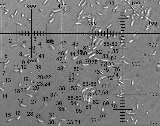 |
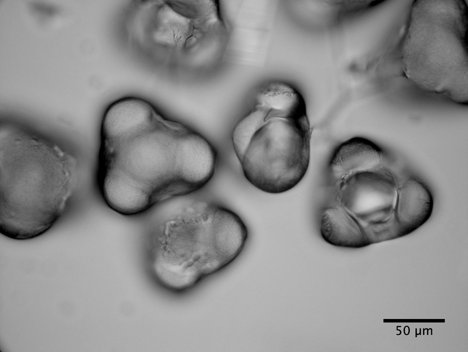
| Clarkia pulchella pollen contents after dehiscence. The scale is 2 microns per division. |
The next figure shows a photo of C. pulchella particles from pollen after dehiscence. 89 particles in the lower left quadrant were labeled and their lengths were measured. A graph of number of particles per radius bin (radius R = 1/2x(particle length), bin size =.25 microns) for both photos appears in the following figure.
Qualitatively, this confirms what Brown said. There are very few
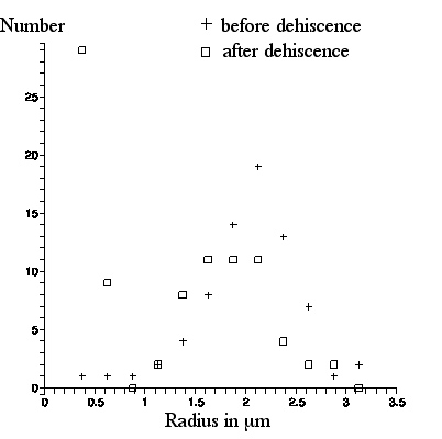 |
| Number of particles (in radius bin .25micron wide) vs. radius in microns. |
spherosomes visible in the picture taken from pollen before dehiscence. The appearance in the picture taken after dehiscence, of many particles of size less than a scale division (the "`molecules" or spherosomes that so excited Brown), is strikingly apparent. These particles appear as light or dark, depending upon their location with respect to the microscope focal plane.
Consider the graph of what is observed in these figures. The distribution of numbers of particles with radii above 1 micron before and after dehiscence appears to be the same: these are the amyloplasts. However, there is a peak in the number of particles with radii less than 1 micron after dehiscence (and no such peak before dehiscence): these are the spherosomes.
Quantitatively, there is a discrepancy between Brown's observation of the sizes of the amyloplasts and spherosomes, and what is depicted here: his sizes are larger. As we have noted, Brown quotes the amyloplasts as having average radius R (half the long axis length) ≈3micron, with maximum R ≈ 4micron, whereas with our Olympus microscope, these numbers are ≈2 and ≈3 microns respectively. And, Brown quotes the spherosome radii as ranging from R ≈.65micron to ≈.85micron whereas, with our Olympus microscope, most spherosomes appear to cluster around R ≈ .5(plus or minus .05) micron, with maximum size ≈.65(plus or minus .05) micron.
To resolve this discrepancy in the case of the spherosomes, in the next section, lenses and their effect on the image of a round object are discussed. Essentially, due to diffraction, Brown's lens and the Olympus microscope both enhance the image beyond the actual size of the object, but the Olympus microscope enhances the image less than did Brown's microscope. The theory summarized here is, in the following section, experimentally found to be in good agreement with observations, of polystyrene spheres of known radius, made with the Olympus microscope. Therefore, in the section after that, the theory is applied to observations of spherosomes with the Olympus microscope, enabling estimation of the spherosome size. Then, Brown's observations of the spherosome size enables estimation of properties of his microscope!
Following this discussion of spherosome sizes, the Brownian motion and rotation evinced in the figure above is treated.
Lastly, the construction of a ball lens microscope with power close to that of Brown's lens is presented. Aided by a picture of amyloplasts taken with it, the amyloplast size discrepancy is discussed.
C2. Lenses
Interestingly, Brown's hypothesis and conclusion, of the ubiquity and uniformity of the ``molecules," although wrong, was so stimulating to him that it led to his famous discovery. As mentioned in the Introduction, when he was viewing objects smaller than the resolution of his lens, diffraction and possibly spherical aberration produced a larger, uniform, size.(7)
We now discuss this further, summarizing mathematical results given in Appendices F and G. The main result is the
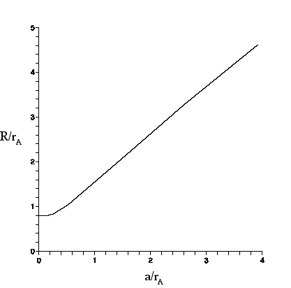 |
| For an circular object of radius a as seen through a lens, R is the radius of the image circle (defined as where the intensity is 5% of the intensity at the center of the image circle). r_{a} is the Airy radius. |
conversion graph shown here, that will enable us to find the radius a of a spherical object from the larger radius R of the image observed through a lens or microscope. The theory shall be compared to observations of polystyrene spheres made with the Olympus microscope. Then, the results shall be applied to the spherosome size discrepancy .
Also, using these ideas, we shall attempt a bit of historical detective work. From information supplied by Brown about the size of his ``molecules," we can hazard a guess at the radius b of the circular aperture that backed his microscope lens, which is called the exit pupil.
For sufficiently small b, a point source of light's image is a diffracted intensity distribution, a circular pattern of light. The intensity as a function of radial distance r from the lens axis is given by the Airy function, Eq. (1):
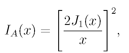
(1)
where J_{1}(x) is the Bessel function and x= krb/f: f is the lens focal length (b/f is called the ``numerical aperture" of the lens), k=2Ï€/lambda, where lambda is the wavelength of the light, traditionally taken for design purposes as green light with lambda=.55micron. This expression (and those which follow) give properly scaled dimensions of the image. Dimensions actually seen through the lens are larger by a factor of the lens magnification.
The Airy function intensity I_{A}(x) is graphed here.
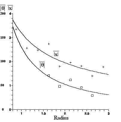
The intensity vanishes at the first zero of the Bessel function, J_{1}(3.83...)=0. This defines the Airy radius r_{A}. Setting kr_{A}b/f=3.83 allows one to find the lens's Airy radius:
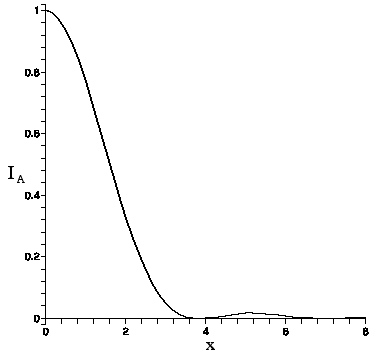 |
| Airy function intensity I_A(x) vs. x |
(2)
Since viewing is subjective, the Airy radius may not be perceived as the boundary of the Airy pattern light intensity (the so-called ``Airy disc"), but it is not far off. For consistency with the non--Airy intensity pattern that appears as b is increased, which also falls off rapidly with distance but does not vanish, we shall define the light boundary as occurring at 5\% of peak value. Applied to the Airy function, since I_{A}(3.01..)=.05, this criterion puts the radius of the light boundary at R= (3.01/3.83)r_{A} or ≈ .8r_{A}.
As b grows, according to Eq. (2), the Airy radius r_{A} diminishes: this increases resolution. Moreover, as the aperture grows, more light exits the lens: this increases visibility.
However, eventually as b is increased further, visibility and resolution start to decrease. The light intensity outside r_{A} grows, and light intensity inside r_{A} decreases. This is due to spherical aberration: rays at the outer edge of the exit pupil come to a focus closer to the lens than do paraxial rays. A design choice, called the Strehl criterion,(8) suggests an optimal choice of b which keeps spherical aberration at a tolerable minimum while maximizing visibility. This criterion is that the intensity on the optic axis (in the image plane that minimizes the observed disc radius) should be 80\% of I_{A}(0). The intensity shape is then still close to the Airy distribution. In this case, the image is described as "diffraction limited": this shall be assumed hereafter.
Consider now, instead of a point source, an extended object, modeled by a hole of radius a illuminated by incoherent light. In geometrical optics, for an ideal lens, each point on the object plane is imaged onto a point on the image plane. Therefore, there will be a circular image which appears also to have radius a. But, with an actual lens, each point in the object plane becomes an Airy disc in the image plane. These discs add like little spotlights of radius r_{A}, with centers uniformly distributed throughout a circle of radius a. Therefore, the image radius R is larger than $a$.
The graph (above) of R/r_{A} vs a/r_{A} was obtained by numerical evaluation of Eq. (28) in Appendix G, which gives the net intensity of the image pattern at any radius in the image plane. The graph can be understood as follows.
For small a, a/r_{A} ≤.25, the centers of the Airy discs that contribute to the intensity are so close together that the intensity is essentially the Airy pattern. Thus, R/r_{A} ≈ .8 as discussed above.
As a/r_{A} grows beyond ≈.25, R starts to grow as well, since the Airy disc centers are now spread out over a non-negligible range. For example, we see from the graph, for a/r_{A} ≈ .5$ that R/r_{A} ≈ 1, and for a/r_{A} ≈ 1, that R/r_{A} ≈ 1.5.
For very large a/r_{A}, the intensity at the center of the image circle is contributed mostly by Airy discs whose own centers lie within an Airy radius of the center. This is true for points somewhat farther out from the center so, at the center and to an extent beyond, the intensity remains essentially constant. But, at distance a-r_{A} from the center, the intensity starts to drop.
At the ``edge" (distance a from the center), the intensity is about half that in the center, because only Airy discs on the inner side of the edge contribute. The intensity drops off further as the distance from the center increases beyond a, reaching 5\% of I_{A}(0) at distance R= a +r_{A}. Thus (R-a)/r_{A} asymptotically approaches 1.
In the graph, R/r_{A} has its largest value for a/r_{A}=4, at which (R-a)/r_{A} ≈.7$. Not shown on the graph are points (a/r_{A}, ≈(R-a)/r_{A)=(8,.8), (17,.9), (30,.99).
C.3 Polystyrene Spheres
To provide an experimental counterpart to these calculations, slides of .3micron and 1micron diameter polystyrene spheres(9) ( diameter standard deviation less than than 3%) were prepared and digitally photographed using our Olympus BX-50 microscope, along with a scale whose line spacing is 2micron. For this microscope, the manufacturer states the resolution is r_{A}=.45micron.
For .3micron diameter spheres, since a=.15micron and so a/r_{A}=.33, we find from the graph that R/r_{A} ≈ .86. Therefore, the spheres should appear as of diameter 2R ≈ 2(.86r_{A}) ≈ .77micron.
No pictures shall be given here, but the observations are summarized. The digital image was enlarged until it appeared as composed of pixels, each a .2micron x .2micron square. Spheres which stood alone (for, many spheres cluster) typically appeared as 3x3 pixel grids (dark in the middle, and grey on the outside, with the surrounding pixels lighter and more-or-less randomly shaded), although a 4x4 grid for a few could not be ruled out. Thus the spheres appeared to be of diameter approximately .6micron, with error of a pixel size, consistent with the estimate.
For 1micron diameter spheres, since a=.5micron and therefore a/r_{A}=1.1, we find from the graph that R/r_{A} ≈ 1.7. Therefore, the spheres should appear as of diameter 2R ≈ 2(1.7r_{A}) ≈ 1.5micron.
In the unenlarged photograph, isolated spheres seemed to be only slightly larger than 1micron, perhaps 1.2-1.3 micron, with a bright center (the spheres are transparent) and dark boundary. However, when enlarged so that the pixels could clearly be seen, particularly the outermost light grey ones, the spheres typically appeared as an 8x8 grid. Thus the spheres appeared to be of diameter 1.6micron, with error of a pixel size, consistent with the estimate.
C.4 Spherosome Sizes and Brown's Lens
In the previous section we have seen that the polystyrene sphere sizes observed through our Olympus microscope are larger than the actual sizes. Therefore, we expect the same to be true of the spherosome sizes. Moreover we expect that the spherosome sizes observed by Brown will be even larger than what we observed, due to a larger Airy radius for Brown's lens than the .45 $\mu$m Airy radius for the Olympus microscope. The universal size of Brown's ``molecules," regardless of their source, can be attributed to their being small enough so that their Airy disc is what Brown observed.
We do not have an electron microscope picture of spherosomes to indicate their actual sizes, as that proved to be very difficult to obtain: that is a challenging project for the future. Unlike amyloplasts which are structurally robust and whose electron microscope picture we succeeded in obtaining (see below), spherosomes are membrane bound lipid droplets: when an attempt is made to concentrate them by filtering so that there are sufficient numbers to view, they coalesce, and appear as an amorphous mass.
We therefore turn to estimate the actual spherosome sizes using our observations through the Olympus microscope As we have noted, according to our graph of number of particles vs. radius above, we observed that most spherosomes appeared to cluster about 1(plus or minus .1)micron in diameter, the largest being perhaps 1.3(plus or minus .1)micron in diameter.
Therefore, for the smallest spherosomes, we have R/r_{A} ≈ (.9/2)/.45 ≈ 1. From our conversion graph we read that a/r_{A} ≈ .5, so their radius is a ≈ .5x.45 or ≈.2micron, i.e., diameter ≈ .4micron.
For most spherosomes, we have R/r_{A} ≈ (1/2)/.45 ≈ 1.1. From our conversion graph we read that therefore a/r_{A} ≈ .6, so their radius is a ≈ .6x.45 ≈ .27micron, i.e., diameter ≈ .54micron.
For the largest spherosomes, we have R/r_{A} ≈ (1.4/2)/.45 ≈ 1.6. From our conversion graph we read that therefore a/r_{A} ≈ 1.1, so their radius is a ≈ 1.1x.45 or ≈ .5micron, i.e., ≈ 1micron.
Armed with these results, we may try to find some properties of Brown's lens.
We assume that the minimum size of his ``molecules" corresponds to the Airy disc, i.e., they belong in the realm $a/r_{A}<.3 for which R/r_{A} ≈ .8$. Since Brown quotes the minimum diameter of his ``molecules" as ≈ 1/20,000in ≈ 1.3micron, half this is the radius R ≈ .65micron, and so the Airy radius of Brown's lens is deduced to be
r_{A}=R/.8 ≈.65/.8 ≈ .8micron.
Then, from Eq. (2) we may conclude that the radius of the exit pupil of his f=1/32 in ≈ .8mm lens was
b=.61x lambda x f/r_{A}}=.61x.55x.8/.8 ≈ .35 mm.
As a consistency check, we note that Brown quoted the maximum diameter of his "molecules" as ≈ 1/15,000in ≈ 1.7micron. Then, R/r_{A} ≈ (1.7/2)/.8 ≈ 1.1. From our conversion graph, we read that this corresponds to a/r_{A} ≈ .6. Therefore, we deduce that the actual radius of these largest spherosomes is a ≈ .6x.8 ≈ .5micron. This agrees with the actual radius of the largest spherosomes we observed.
This concludes our investigation into spherosome sizes
C.5 Amyloplast Brownian Motion and Rotation
We next turn to analysis of the observed Brownian motion of the amyloplasts. In what follows, R iis half the length of the long axis of an amyloplast.
From the figure in Section C.1 which displays two photographs of Clarkia pulchella pollen contents before dehiscence, taken 1 minute apart, the x--displacement, y--displacement, and theta--displacement of each amyloplast, over the one minute interval, were found using the program ImageJ.(6) Because of the possibility of overall fluid flow (assumed constant and irrotational in the region containing the observed particles), the mean displacement was calculated; it proved to be .053micron in the x-direction (negligible flow) and -.847 micron in the y-direction. This was then subtracted from each displacement, to give the true Brownian contribution.
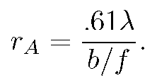
A plot of mean linear displacement and a graph of mean angular displacement for each R bin (.25micron wide) appears below. Smallest and largest R values representing too few data points were omitted.This figure was made with the Maple program (with labeling help from the Appleworks program), and includes graphs of the least squares fit to a power law A/R^{B} for each set of data.
 |
| Mean linear displacement in microns and mean angular displacement in degrees, vs. R in microns (for amyloplasts from C. pulchella undergoing Brownian motion for 60sec). The least squares fit curves are given in the equations nearby. |
The results, compared with the predictions given in Section IIIC are:
The powers in the compared equations agree reasonably well, considering that no correction has been made for the ellipsoidal nature of the particles. (As discussed in Section IIIB and Appendix B, R_{eff} for translation and rotation of ellipsoids should be less than R for a sphere by a factor that is different for the long and short axes, and that varies with their ratio. No attempt was made to correct for this effect, nor for the fact that the observed amyloplast sizes are larger than the actual sizes, just as in the case of the spherosomes.
Interesting studies, with appropriate selection of uniform particle sizes, can be made. The subject of Brownian motion of ellipsoids, first studied by Perrin, is still of interest.(10)
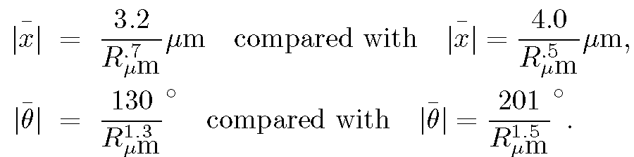
The numerical coefficients in the compared equations differ because the last terms on the right--hand sides of the equations in Section IIIC assume the fluid in which the particles are immersed is water. However, the amyloplasts move in a fluid that is a mixture of water and the intracellular medium, which emerged with the amyloplasts from the pollen. That is, the measured coefficients are proportional to the inverse square root of the viscosity of the fluid, whereas while the expressions shown above are proportional to the inverse square root of the viscosity of water. From the displacement expressions above we obtain for the square root of the ratio of viscosity of fluid to the viscosity of water the value (4.0/3.2) or approximately 1.3, while from the angular displacements this is (201/130) or approximately1.5. These estimates of the fluid viscosity are in reasonable agreement, especially considering the omission of an ellipsoidal correction mentioned above.
One last qualitative observation is worth mentioning. Some wet-dry 400 grit sandpaper was used to grind to powder some of a seashell, a rock, and a nickel. In all cases, the powder (which was colored white or grey, while the sandpaper was colored black, so the sandpaper grit was not being observed), had some particles of apparent sizes < 1micron which were observed jiggling in water, just as Brown said occurred for anything he ground up fine enough.
D. Ball Lens Microscope
Finally, we discuss construction of a single lens microscope with a magnification comparable to Brown's, and some observations made with it.
Ground lenses of high magnification such as those made by Bancks and Dollond are not readily available nowadays. However, fortunately, precision small glass spheres called ball lenses are readily available (they are used for coupling lasers to optical fibers) that can be used as high magnification lenses.(11) We purchased a ball lens of 1 mm diameter and index of refraction 1.517.(12)
The focal length f of a sphere of radius R can be found from the lensmaker's formula(13) for a thick lens of radii R_{1} and -R_{2}, thickness T and index of refraction n:
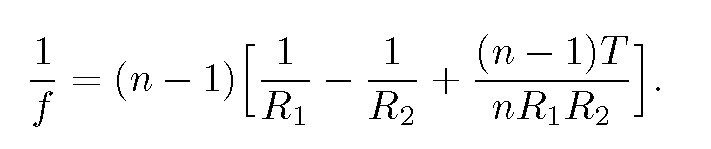
For T=2R and R_{1}=-R_{2}=R, this equation yields
f=nR/[2(n-1)].
For our lens, f= .733 mm=1/34.6 inch, not far from the f=1/32 inch of Brown's lens.
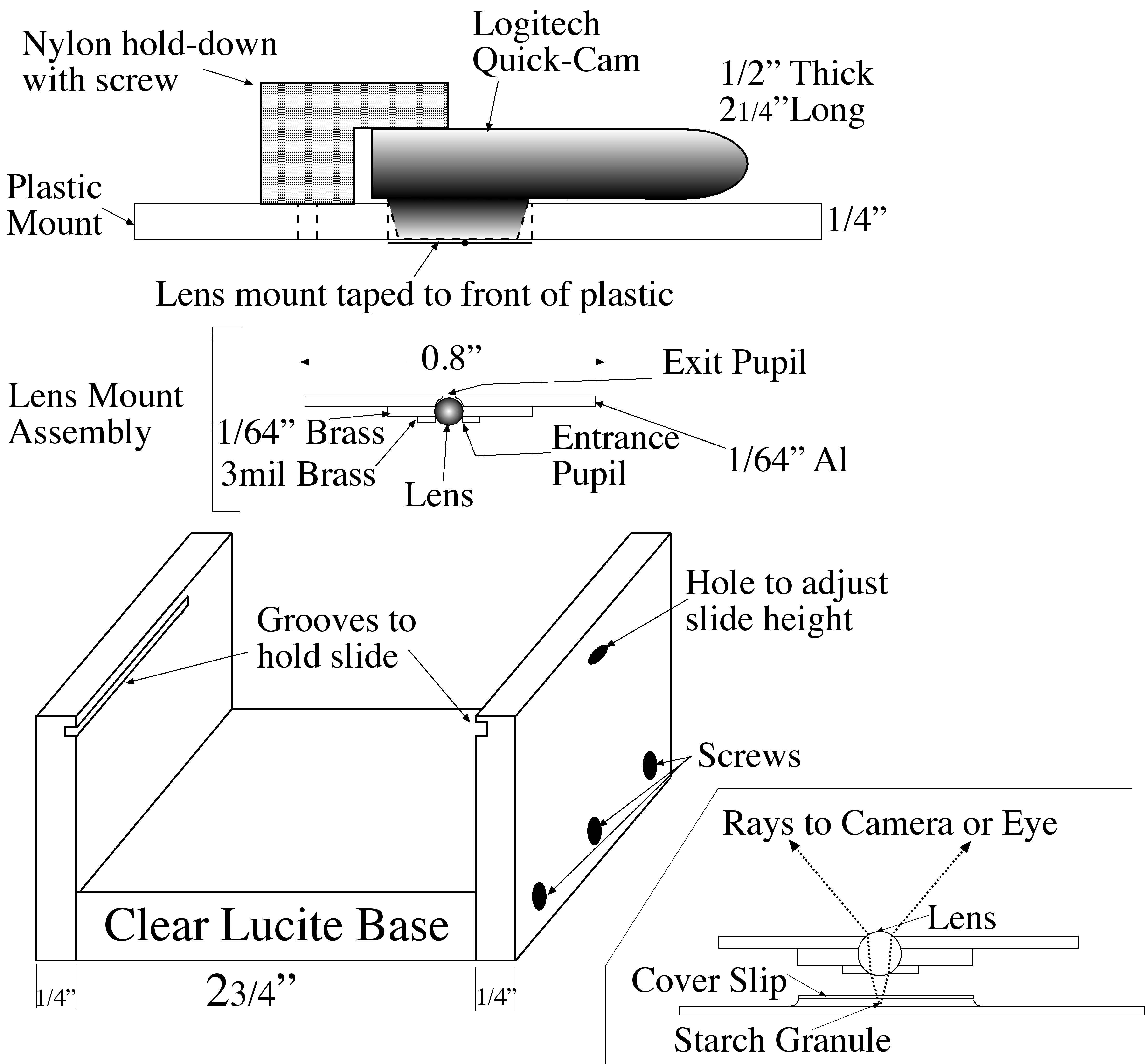
The ``microscope" is essentially the lens sandwiched between two perforated supports. One support was made as follows. A circle of 1" diameter was cut out of a 1/64" (approximately 0.4 mm) thick aluminum sheet. A 0.8 mm. diameter hole was drilled part way through its center, and then a 0.48 mm diameter hole was drilled all the way
 |
| Microscope Diagram |
through. Thus, the exit pupil radius was constructed to be 0.24 mm. Then, a small washer was made from a piece of 1/64" brass with a 1 mm diameter hole drilled through it. The holes in the two pieces were aligned, and the pieces secured to each other with Kapton polyimide tape. The ball lens was placed in the resulting hole, supported by the edges of the 0.48 mm hole and surrounded by the washer.
The second support consisted of a piece of 3 mil (0.076 mm) brass shim stock with a 0.55 mm diameter hole in the center, It was secured over the lens with more Kapton tape to hold the lens in place and serve as the entrance aperture.
The assembled ``microscope" was then mounted with more Kapton tape over the entrance aperture of a Logitech QuickCam Pro USB camera. This camera was chosen from a large number of such ``webcams" because the front of its lens lies very close to the surface of the camera, allowing a very small separation between the microscope and the imaging camera. A 1/4" x 3" x 5" plastic sheet was fashioned, and a hole was drilled through its center, through which the microscope backed by the camera lens protrudes: the body of the camera rests upon the plastic. An inverted-L shaped bracket was attached to the plastic sheet to hold the camera .
A U-shaped plastic stand, of dimensions slightly less than 3" (the length of a microscope slide) was constructed from 1/4" plastic. Horizontal grooves (rabbets) to support the slide were cut in the sides of the U just below the top edges. The plastic sheet holding the microscope/camera rests upon the top edges of the U, and can be moved frerely over the slide.
 |
| Ball lens microscope |
A small hole was drilled through one side of the U, partly through and partly below the rabbet. Focus adjustment is achieved by placing a small wedge (e.g., a toothpick) through the hole and under the slide. As the wedge is moved in and out, it raises and lowers the slide by a fraction of a millimeter. Light from a small microscope illuminator, collimated to a 1" beam, is diffusely reflected from a white surface on which the plastic stand sits, through the slide and into the microscope/camera.
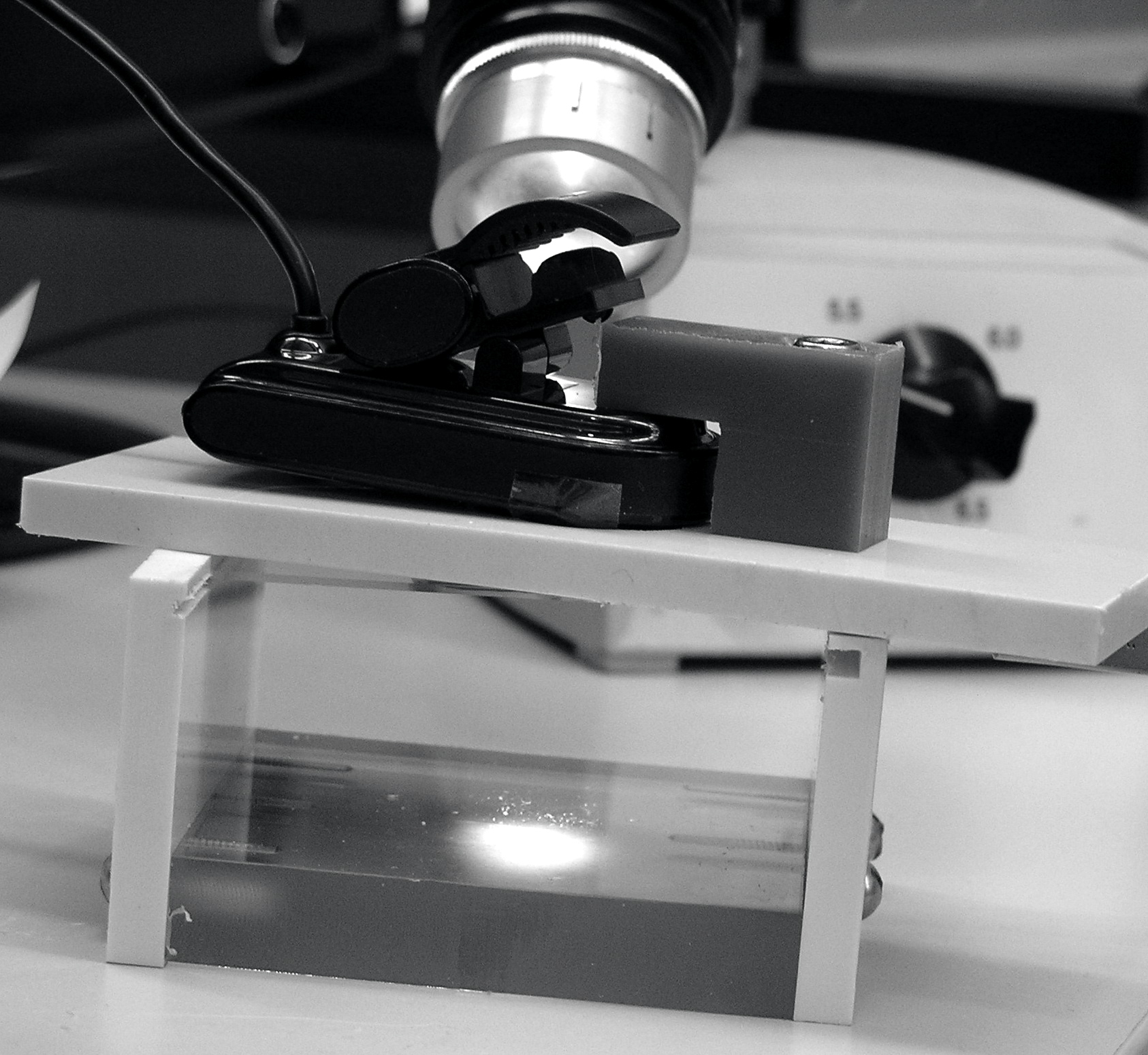
In the photograph of the microscope, the plastic sheet supporting the camera (whose cable goes off to the left) lies in the middle of the picture, slightly skewed to the stand. The ball lens and its support, attached to the camera aperture, lies within a hole in the middle of the plastic sheet, and so is not visible, nor is the focus adjustment hole in the side visible. The inverted L-shaped bracket that affixes the camera, the rabbets which support a slide, and a bit of a slide itself (just below the plastic sheet on the left), the inverted U stand, as well as the light source and its power supply, are visible.
E. Amyloplasts Seen With Ball Lens Microscope
Now we address the discrepancy between our observations with the Olympus microscope, that the amyloplasts appear to be of average radius (i.e., half-length) about 2micron, with maximum radius about 3micron, and Brown's observations with his microscope, that their radius range is about 3--4micron. We shall do so by showing that the
 |
| Clarkia pulchella amyloplasts photograped with the electron microscope |
observations with the ball lens are essentially the same as Brown's. But, also, we have taken an electron microscope picture of amyloplasts which, while not depicting a large sample, suggests that the size distribution measured with the Olympus microscope is reasonably accurate.
For the ball lens, the Airy radius is r_{A}=.61(llambda)f/b=1.0micron. The exit pupil b=.24mm is not the ideal size to minimize spherical aberration according to the Strehl criterion (discussed earlier). That ideal size is b=.19 mm. However, its intensity is still reasonably approximated by the Airy function, so we shall assume that the considerations leading to our conversion graph of R/r_{A} vs. a/r_{A} above are valid.
To check that r_{A}=1micron for the ball lens, a slide containing 1 micron diameter polystyrene spheres was observed and photographed. Another slide containing a scale with marks 10micron apart was separately photographed. Both photographs were superimposed using the program Photoshop Elements 2. Using the program ImageJ, the image of the spheres was enlarged so that the pixels could be seen, and they were analyzed, as described earlier for the spheres photographed with the Olympus microscope. The result was that the polystyrene spheres appeared to have diameter 2.1(plus or minus.2)micron.
 |
| Clarkia pulchella Amyloplasts photographed with the ball lens microscope. The superimposed scale marks are 10micron apart. |
For a theoretical comparison, with a/r_{A}=.5/1=.5, one reads from our conversion graph that R/r_{A}=1.1. Therefore, it is predicted that the apparent radius of the spheres should be R=1.1r_{A}=1.1micron, or diameter 2.2micron, in good agreement with the observation discussed above.
Now we turn to compare the amyloplast sizes seen with the Olympus microscope and amyloplast sizes seen through the ball lens. The figure to the left shows a portion of a photo taken through the ball lens, of a slide containing amyloplasts that had emerged from a pollen grain (whose out-of-focus edge appears at the lower left).
A a photograph of a scale with 10 micron mark separation was superimposed and the photograph was further enlarged so that pixels were visible. The radius (half the length) of 44 amyloplasts was measured, 14 of which appear in this picture and 30 appear in another photograph of a different scene. Below we present a graph of the number of amyloplasts in a .25micron radius bin versus amyloplast radius in microns.
From this graph, the amyloplasts appear through our ball lens as of average radius about 3micron, with maximum radius about 4micron.
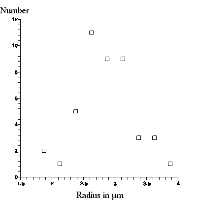 |
| Number of amyloplasts, seen with the ball lens, in a .25micron bin vs. amyloplast radius. |
This is about 1micron larger than what was observed with the Olympus microscope, but exactly what Brown said about the amyloplast sizes he observed through his lens!
This excellent agreement, between the observations with our ball lens and Brown's observations with his lens should be tempered by the realization that our lens has r_{A}=1micron and exit pupil b=.24mm, whereas we have deduced that Brown's lens had r_{A}=.8micron and exit pupil b=.35mm. However, it leaves little doubt that Brown was seeing enlarged amyloplasts on account of the diffraction and possible spherical aberration of his lens.
-----------------------------------------------
Acknowlegments
It is a pleasure to thank Diane Bilderback, Brent Elliot, Brian Ford, Armando Mendez, Michael Milder, Bill Pfitsch, Hilary Joy Pitoniak, Diana Pilson, Bronwen Quarry, James Reveal, Ann Silversmith, Ernest Small, and David Mabberley for help with this endeavor.
---------------------------------------------------------------------------------------
1) H. Lewis and M. E. Lewis, The Genus Clarkia (University of California Publications in Botany 20, pp. 241-392, 1955), p. 356.
2) I grew Clarkia plants from Diane's seeds, http://www.dianeseeds.com: packets of C. pulchella (containing approximately1000 seeds), C. amoena (approximately1800 seeds) and C. elegans (approximately 1500 seeds) each cost $2.00. Everwilde farms, http://www.everwilde.com sells packets (approximately 2000 seeds) of the latter two species for $2.50. Thompson and Morgan, http://www. tmseeds.com, a British company, sells packets of C. pulchella and C. elegans (approximately 400 seeds) for $2.55. Monticello sells a packet of seeds of C. pulchella (a plant cultivated by Thomas Jefferson) for $2.50, but I did not have good results with these seeds.
3) The U. S. Department of Agriculture site, http://plants.usda.gov/, has much general information on species. Under Scientific Name, type in Clarkia, and then choose Clarkia Pursh.
4) http://www.leevalley.com. The Lee Valley Seed Starter costs $22.50 plus shipping. One can purchase 25 plastic pots for \$9.50, and a plastic tray which holds 24 such pots for $26.50.
5) Hydrofarm Green Thumb or Jump Start (they seem to be the same) fixtures with bulbs are available from various vendors. For example, DirtWorks, http://www.dirtworks.net/Grow-Lights.html, sells the fixture, the 2 foot version (which will light one Lee Valley Seed Starter) costs $69 plus shipping and the 4-foot version (which I bought and which lights three Lee Valley Seed Starters) costs $89 plus shipping.
6) ImageJ is available from the National Institutes of Health web site http://rsbweb.nih.gov/ij/.
7) P. W. van der Pas, Scientiarum Historia 13, 127 (1971). Of Brown's molecules, van der Pas says: `` ... they were approximately of the same size; their diameter varying between 1.26 and 1.6 microns. These statements are not true, BROWN was led to them because he worked with an imperfect lens at the border line of its magnifying power." This was the only placein the literature where we could find a remarkn about the effect of Brown's lens.
van der Pas did not enlarge upon this point. He wrote his paper to call attention to a rather throw-away paragraph in a paper in 1784 by Jan Ingenhousz, thereby intimating Ingenhousz's priority over Brown. The purpose of Ingenhousz's paper was to introduce the idea of a transparent cover slip in microscopy to prevent water evaporation. Unlike others who had seen Brownian motion before Brown, but attributed it to life, Ingenhousz observed and clearly asserted in this paragraph that nonliving matter underwent the motion, but he did no systematic investigation.
Citing van der Pas, Mabberley D. J. Mabberley, Jupiter Botanicus: Robert Brown of the British Museum (J. Cramer, Braunschweig 1985), p. 272, says: ``It has been shown that Brown's 'molecules' were artifacts, there being no particles 1.26-1.6micron across in pollen grains or elsewhere." However, this statement is only partially correct. While there are not universal particles of this size range as Brown supposed, spherosomes imaged to such size were certainly seen by Brown. Spherosomes have been observed in various plant tissues of diameter .4-4micron: see T. J. Jacks, L. Y. Yatsu and A. M. Altschul, Plant Physiol. 42, 585 (1967); L. Y. Yatsu,
T. J. Jacks and T. P Hensarling, Plant Physiol. 48, 675 (1971).
8) K. W. A. Strehl, Zeit. fur Instr. 22, 213 (1902). The Strehl criterion is mentioned in most books on optical design, e.g., D. Malacara and Z. Malacara, The Handbook of Optical Design, 2nd Edition (Marcel Dekker, New York 2003), p. 211.
9) The polystyrene latex spheres were obtained from Ted Pella, Inc., http://www.tedpella.com/.
10)F. Perrin, Journ. Phys. Radium V, 497 (1934); R. Vasanthi, S. Rarichandran and B. Bagchi, Journ. Chem. Phys. 114, 7989 (2001); Y. Han et. al., Science 314, 626 (2006).
11) Two web sites that describe construction of such microscopes are http://www.microscopy-uk.org.uk/mag/artjul06/aa-lens3.html and http://www.funsci.com/fun3_en/usph/usph.htm#0.
12) Edmund Optical Company, 1 mm diameter ball lens #NT43-708, costing $22, http://www.edmundoptics.com/onlinecatalog/displayproduct.cfm?productID=2041&PageNum=1&StartRow=1.
13) A. C. Hardy and F. H. Perrin The Principles of Optics (McGraw-Hill, New York 1932), p. 58, Eq. (71).