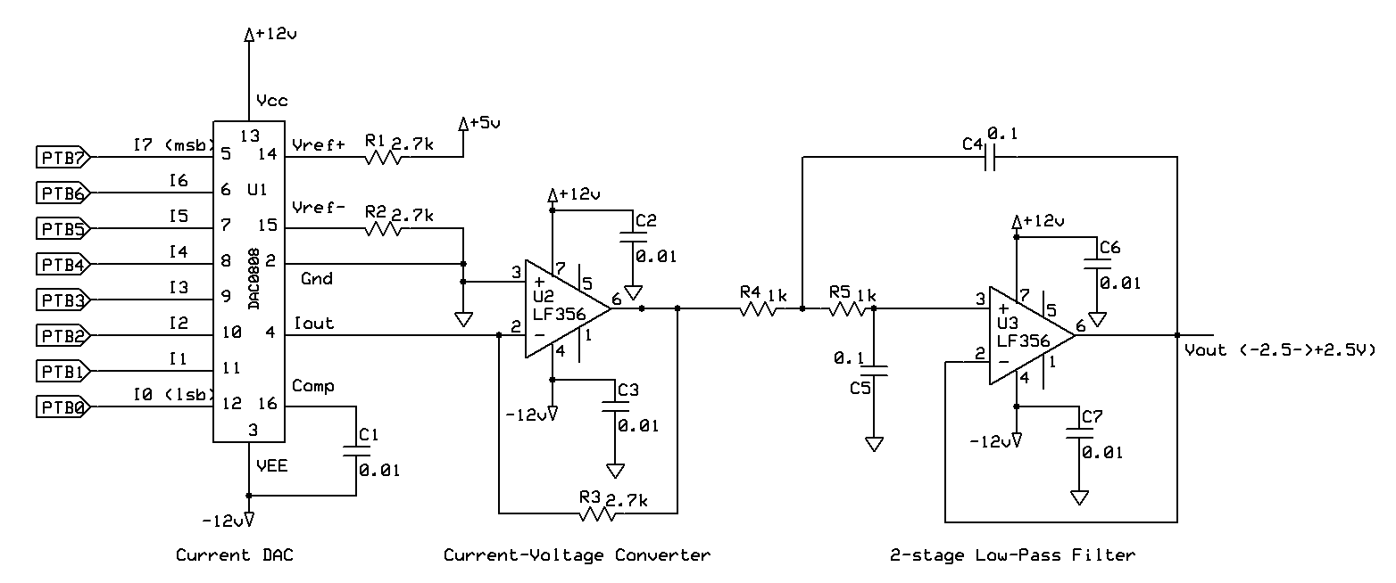
The best way to create sound with a computer is to send a sequence of numbers to a DAC where they are converted to voltages that can be amplified and sent to loudspeaker. A musical sound is a smoothly varying sound pressure wave that varies with a range of frequencies between about 20Hz and 20,000Hz. An amplifier and loudspeaker can convert a smoothly varying voltage to a smoothly varying sound pressure so all we need is to create the smoothly varying voltage, which we can approximate with a DAC and a low-pass filter.
The hardware for this is quite straightforward.
The voltage coming from the DAC looks rather like a noisy staircase. Every time we send a new value the output voltage wobbles around (switching noise) and then settles to a new steady value. However, we would like the output voltage to vary smoothly. We can improve this by adding a low-pass filter to the DAC. Even a very simple RC filter can provide a significant improvement if the values are chosen well. We want to pass through frequencies that could be part of the signal but block the higher frequencies that contain information about the steps and the noise.
Let’s look at a very simple example. Consider sending an arithmetic sequence to DAC, 0,1,2,3,4, and so on. The output from an idea DAC would be a perfectly regular staircase and the ideal smoothed output would be a perfect straight line. This is something that we can analyse. The math is a little fiddly but it is straightforward to show that the result of putting the staircase in figure 1a below through a single section RC low-pass filter with its cut-off at the sample frequency is the slightly wiggly straight line in figure 1b. If we look at the difference between the output and a real straight lines (figure 1c) we see that, after a starting transient, the error settles down to about 1/10th of a step in magnitude (the half step constant error is just a bad choice of origin–it has no audible effect since it does not vary).
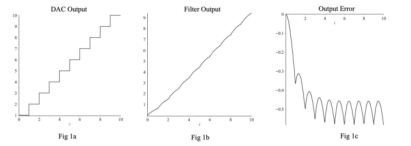
So, even a single section RC filter gives impressive results. In practice I included a two-section Sallen-Key low-pass filter which gives even better results as you you can see in this figure.
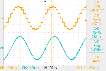
The upper trace (yellow) is the output of the DAC and it clearly shows the large steps from which our sinewave is approximated. The lower (cyan) trace is the output of the filter. It is indistinguishable from a sinewave by eye and also to my ear.
The simplest possible musical sound is a pure sinewave. We can generate that by filling a table with numbers generated by a sine function and then sending those numbers to the DAC at a perfectly regular rate. Let’s do a little math!
The first thing you need to know is that there is a rule called the Nyquist theorem that says that the highest frequency that you possibly generate from samples sent at rate R/sec is f=R/2. Thus, if we want to generate all audible sound we should aim for a sample rate of at least 40,000 samples/second. For example, CDs used a sample rate of 44,100 samples/second.
The second key idea is that the more data that we have in the table the better the quality of the output. This shows up in both dimensions, time and number of bits. I will discuss this in more detail at a later time but for now we will be limited by the resolution of the DAC and so need to look only at the effect of table length. The longer the table, the more accurately we will be able to reproduce the sinewave shape and the lower the frequency of the note. If we have a sample rate R and a table with N samples in it then the frequency at which the table repeats, the frequency of the note, will be R/N. So, for example, a 128 entry table with a sample rate of 40,000/second will give us a note frequency of f = R/N = 40,000/128 = 312.5Hz. That corresponds to a note near the Eb above middle C in the standard A440 scale. A 16-entry table will give the note 4 octaves above that, f = 40,000/16 = 2500Hz.
So we have our first recipe to produce a single pure frequency tone! Fill a table of 128 values with numbers generated from a sine function and play them out one at a time at a rate of 40,000 samples per second.
A sine function takes real number values from –1.0 to +1.0 and thus is a terrible match to an 8-bit DAC that requires integer values between 0 and 255. We have to find a way to transform one to the other. With the values shown in the diagram (Figure 1) above the DAC output voltage varies from ??? when set to value 0 to ??? when set to value 255. We can map these onto the sine range of –1 to +1 using the linear transform
DAC = Sine * 127 + 128
which sets DAC to 128 when Sine is 0, to 1 when Sine is –1, and to 255 when Sine is +1. This formula is easy to type into a spreadsheet that can be used to generate all the values for a table in one go. We simply start with a set of angles between 0 and nearly 2*π and tell Excel to truncate the answers to integers. Here is an example spreadsheet for a rather small, 16 entry, table.
| Wavetable Spreadsheet | ||||
| Number of table entries | 16 | |||
| Index | Angle (rad) | Sine(Angle) | DAC # | DAC Integer |
| 0 | 0 | 0 | 128 | 128 |
| 1 | 0.392699082 | 0.382683432 | 176.6007959 | 176 |
| 2 | 0.785398163 | 0.707106781 | 217.8025612 | 217 |
| 3 | 1.178097245 | 0.923879533 | 245.3327006 | 245 |
| 4 | 1.570796327 | 1 | 255 | 255 |
| 5 | 1.963495408 | 0.923879533 | 245.3327006 | 245 |
| 6 | 2.35619449 | 0.707106781 | 217.8025612 | 217 |
| 7 | 2.748893572 | 0.382683432 | 176.6007959 | 176 |
| 8 | 3.141592654 | 1.22515E-16 | 128 | 128 |
| 9 | 3.534291735 | -0.382683432 | 79.39920409 | 79 |
| 10 | 3.926990817 | -0.707106781 | 38.19743879 | 38 |
| 11 | 4.319689899 | -0.923879533 | 10.66729937 | 10 |
| 12 | 4.71238898 | -1 | 1 | 1 |
| 13 | 5.105088062 | -0.923879533 | 10.66729937 | 10 |
| 14 | 5.497787144 | -0.707106781 | 38.19743879 | 38 |
| 15 | 5.890486225 | -0.382683432 | 79.39920409 | 79 |
| Formulae | ||||
| Angle (rad) | "=2 * PI() * A6 / $C$3" | |||
| Sine(Angle | "=SIN(B6)" | |||
| DAC # | "=C6*127+128" | |||
| DAC Integ | "=TRUNC(D6)" | |||
It is then a simple matter to copy the contents of the “DAC Integer” column into our source file to initialise a table.
const char gWave[16] = {
    128, 176, 217, 245, 255, 245, 217, 176,
    128, 79, 38, 10, 1, 10, 38, 79
};
and all I had to do was add the commas and remove some of the newlines to compress it onto fewer lines. For larger tables it is easier just to let the table run to as many lines as it wants.
Since the output frequency is set by both the sample rate and the length of the table it appears that we could change the frequency by altering either. In practice these lead to very different tradeoffs between complexity and quality.
In this method we keep the wave table fixed and play with the sample rate to adjust the frequency.
The basic job of sending the table out is simple, just work through the table entries one at a time waiting an appropriate time between each. For the table above we get something like
char index = 0;         // Will run through 0-15 indices of array

void setup(void) {
    portMode(PORTB, OUTPUT);    // Assuming DAC on PORTB
}
void loop {
    portWrite(PORTB, gWave[index]); // Send next sample
    index = (index + 1) % 16;               // Modulo operation makes sure in domain 0-15
}
If we actually do this then a number of problems appear.
First, we have not even tried to control the loop speed. Instead of giving us a frequency
of 2500Hz the output is actually at about 13.3kHz. We need to try to slow the rate
a little. The shortest delay routine that we know, delayMicroseconds, is the obvious
choice. Here is an updated version of the program with that added. I have made the
length of the delay adjustable. Since we want to output 40,000 samples per second that
should give us a duration for each sample of 1/40,000 = 25uS.
char index = 0;         // Will run through 0-15 indices of array
char nSLow = 25;        // Number of microseconds to wait between samples

void setup(void) {
    portMode(PORTB, OUTPUT);    // Assuming DAC on PORTB
}
void loop {
    portWrite(PORTB, gWave[index]); // Send next sample
    index = (index + 1) % 16;               // Modulo operation makes sure in domain 0-15
    delayMicroseconds(nSlow);
}
Because there is some overhead to the loop this does not work quite as expected. Instead of 40,000 samples per second and a frequency of 2,500Hz I got ???.
I experimented with different values for the loop delay and got these results
Delay   Frequency
    10  3874Hz
    20  2385Hz
    19  2480Hz
    18  2584Hz
and clearly we won’t do any better than that! At 19 we are off by –4.8%, which corresponds to a little less than 1 semitone flat, while at 18 we are about 3.3% high, almost half a semitone sharp.
This all means that we can’t get nearly enough frequency resolution this way, let alone accuracy.
Even if we had been lucky and had been able to get the correct frequency we would still have a problem. Looking at the signal with an oscilloscope it is easy to see that the frequency is not constant. Instead, the period wobbles around by fractions of a microsecond. This is because the time between samples is not uniform. There is some overhead associated with the loop that varies between trips. It takes longer every time we reach index=16 and have to reset the index. This jitter makes this a poor method for producing quality sound.
This one is actually quite easy to get rid of. All we have to do is make each loop
identical. The point of the inner for loop is to prevent index from exceeding
15 = 0x0f. The hex view gives a better solution. If we AND the index with 0x0f before
using it then we can be assured that index & 0x0f always lies in the domain [0–15],
exactly as we wish. This gives us the code
void main(void) {
    char index = 0;         // Will run through 0-15 indices of array
    char delay;                 // Delay loop counter
    portMode(PORTB, OUTPUT);    // Assuming DAC on PORTB
    for (;; index++) {
        portWrite(PORTB, gWave[index & 0x0f]);          // Send next sample
        for (delay = 0; delay < 100; delay++) {};
    }
}
NOTE that I used the increment slot of the main for loop to increment index. I could just have done it in the loop but this seems more in keeping with C. With that change I get no visible jitter on the scope and slightly higher frequencies
Delay   Frequency
    10  4139Hz
    20  2483Hz
If you just want a limited selection of notes then this is a useable, and very simple to program method of note generation. If we settle for a lower sample frequency then we can use longer delays and improve the frequency resolution. We will not be able to closely match the low-pass filter cutoff to the sample rate since the sample rate will vary from note to note so our sound quality will be markedly poorer as well as our note choice being limited. But it is certainly good enough to play a simple tune as we will see if we look at much larger delays.
For example, if we go to delays near 200 we get much finer tuning.
Delay   Frequency
200 301.4Hz
201 299.9Hz
202 298.5Hz
Here the frequency differences are at the 0.5% level or about 1/10 of a semitone. It is quite easy to produce more than one octave of pitches that sound well-tuned to the average ear. That leads us to the problem of choosing frequencies for our notes.
We can look up the standard frequencies for musical pitches. The set of frequencies most commonly used today is called the equal tempered scale and is based on splitting the octave (two frequencies with the property that f2 = 2 * f1) into 12 equal semitones. If we combine that idea with the standard choice of a reference pitch, A4=440Hz, then we get the following formula for the pitches of other notes
fn = 440 * 2<sup>n/12</sup>
where n is number of semitones above A4 that we seek. Thus we can find the frequency for middle C (C4), which is 9 semitones below A4, by
fC4 = 440 * 2<sup>-9/12</sup> = 440 / 2<sup>3/4</sup> = 261.63Hz (5 s.f.)
That is about 40Hz below 301.4Hz and each increase of 1 the delay was adding about 1.5Hz to the frequency of the note in our text so I will start to look near 200 + 40/1.5=227.
Delay   Frequency
227 266.4Hz
229 264.2Hz
231 261.9Hz
That is only 0.3Hz sharp, about 1/20 of a semitone.
For reference here is a table of pitches and their frequencies.
Now we know how to create individual pitches we can try to combine them into tunes. It would clearly be very useful to have a subroutine that would play a given pitch for a given length of time. Since the delay is the only thing that changes from pitch to pitch we could pass the delay to a subroutine along with a number of samples to play. That would give us something like this.
void PlayNote(char delay, int nSample) {
    int s = 0;
    char d;
    for (; s < nSample; s++) {
            portWrite(PORTB, gWave[index & 0x0f]);          // Send next sample
            for (d = 0; d < delay; d++) {};
        }
    }
}
Interestingly, that gives us completely different frequencies from the previous version!
For example, with a delay of 231 I now get 33.3Hz!!! Somehow this fails to work properly.
I have been unable to figure out why this does not work correctly but the fix turned
out to be simple. If I use a down-counting for loop instead of an up-counter then I get
the code below which works perfectly, though the delay=231 frequency has shifted slightly
to 260.7Hz and delay=230 is now a better choice for C4.
I can now play a simple tune by making calls to PlayNote with different delays and numbers of samples.
It would be nice if PlayNote could be told the pitch to play instead of having to
be given a rather arbitrary delay number. We can make this happen with a table that
maps note number (in some encoding) to delay. For example, if we call note 0 this
C4 and then increase by semitones so that e.g. note 4 is E3, note 5 is F4, and note 7
is G4, then a table that starts like this will work (though mine has very few notes!).
const char gDelay(6) {
    230,  217, 204, 192, 181, 171
};
and we alter PlayNote slightly to get
void PlayNote(char note, int nSample) {
    int s = 0;
    char delay = gDelay[note];
    char d;
    for (; s < nSample; s++) {
            portWrite(PORTB, gWave[index & 0x0f]);          // Send next sample
            for (d = 0; d < delay; d++) {};
        }
    }
}
which is slightly dangerous since you could call it with an out-of-range value for
note and get a random pitch.
The last thing we would like to do is to make the note duration independent of the note. We can do this by computing the number of samples from the duration and the delay value. The duration is (in arbitrary units) the product of nSample and delay. For example, at A440 we have to play 440 * 16 = 7040 samples to last 1 second. The delay for A440 is 134 so that 1 second duration corresponds to 7040 * 134 = 943360. If we will settle for times to the nearest 1/10 second then we can find the number of samples for a given number of 1/10th second units by
nSample = nUnit * 94336 / delay;
If we want slightly more control over our timing then we can use 1/100 second units of time and do
nSample = nUnit * 9434 / delay;
This is slightly less accurate but gives much better precision and allows for much shorter notes. The computation is inconvenient since it requires a 32-bit number to do the arithmetic but it only happens once per note and does not produce a visible delay between one note and the next.
This gives us our final low-quality PlayNote routine.
/*
 *  PlayNote plays a single sine tone for a given note that lasts
 *  nUnit/100 seconds. The notes are coded
 *  0->C4, 1->C#4, 2->D4, 3->D#4, and so on.
 */
void PlayNote(char note, int nUnit) {
    char delay = gDelay[note];
    long duration = nUnit + 9434;
    int nSample = duration / delay;
    int s = 0;
    char d;
    for (; s < nSample; s++) {
            portWrite(PORTB, gWave[index & 0x0f]);          // Send next sample
            for (d = 0; d < delay; d++) {};
        }
    }
}
It is worth noting that we have been able to get a nice range of useful notes in part because I happened to choose a rather short (16-entry) sine table. A longer table would give lower pitches at the same delay (an octave lower for each factor of 2 increase in table length). Thus we have to make compromises between frequency accuracy and signal accuracy with this method.
If we want accurate sample rates and fine control over the range of frequencies available then we need something more complex. In method 1 we changed our frequency by changing our sample rate. This time we will keep the sample rate fixed (which makes our low-pass filter much happier) and play games with the way we read out the wave table.
First we need a method to ensure a perfectly regular sample rate. With current processors this is much easier to achieve in hardware than it is in software. At the heart of the microcontroller there is a very precise clock generator to which all the operations of the chip are synchronized. Most microcontrollers allow us to use the internal to control or measure times to high accuracy. The 9S08GT has two independent sets of hardware timers that will allow us to generate an extremely constant output sample rate.
A timer can provide us an extremely regular source of events, essentially a clock. Such a clock can interrupt the computer and cause a small piece of code, called an interrupt handler, to run at times that are set by that clock and are not subject to variations in how long loops take to run. You can read about interrupt handlers in Chapter 13 of the Computer book.
So the basic idea is to arrange that a short subroutine will be executed at an exact rate based on the ticking of a hardware clock. In that subroutine we find the next value and send it to the DAC. So long as there are values available from somewhere this gives us a way to output sound that is precisely controlled and that has the additional benefit of being able to run in parallel with other code. Thus it becomes possible to, for example, make a robot play a tune while it navigates around the room.
If the sample rate is fixed and the table length is fixed then how do we vary the frequency of the sound? The answer lies in varying the size of step that we take through the table. Let’s take our 16-entry table as an example. At a sample rate of 40kHz with 16 samples per period we output 40,000/16 = 2500 periods per second.
Now, what if we were to leave out all the odd numbered steps and send only the even numbered samples, 0, 2, 4, etc. In that case we output only 8 samples before we repeated and the output frequency would be 40,000/8 = 5000Hz, an octave lower than the original pitch. Of course, with only 8 samples per period our sinewave would be getting pretty choppy looking (figure below) but a good filter would still be able to output a decent sinewave. One way to look at this is to think that instead of adding 1 to the index to get to the new sample now we add 2 each time. We have a stepsize of 2.
Similarly, we could send each sample twice? In that case we would get a slightly choppier looking wave with a longer period. We would now have to send 32 samples to get back to the start so the output frequency would be 40,000/32 = 1250Hz, an octave lower than the previous case. This is like taking two half steps instead of one whole step but always using only the integer part of the step number. So we would have the real step number (possibly fractional) and the table index (an integer), like this
Real 0.0 0.5 1.0 1.5 2.0 2.5 3.0 3.5 ...
Index 0   0   1   1   2   2   3   3  ...
Now what if we picked a different step size. For example 1.5
Real 0.0 1.5 3.0 4.5 6.0 7.5 9.0 10.5 12.0 13.5 15.0 16.5 18.0 ...
Index  0  1   3   4   6   7   9   10   12   13   15    0    3  ...
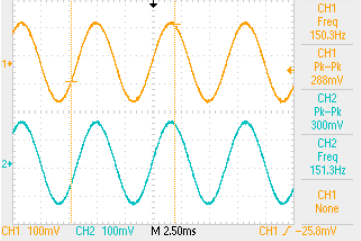
At this point we have been all the way through the table once so we have completed one period but we have sent only 11 samples instead of the 16 samples for a normal wave. If we keep this up then on average we will send 16/1.5 = 10.67 samples period. What does this actually look like? Well here are some oscilloscope traces with the signal before the filter in the upper, yellow, trace and the signal after the low-pass filter in the lower, cyan, trace.
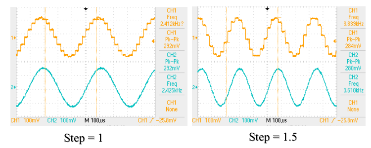
As you see the output looks surprisingly normal. Each period is slightly different from the one before in the details but the general shape is just a sinewave with a frequency of 40,000 / 10.67 = 3750 = 1.5 * 2500Hz! So if I step through the table with non-integral steps I get a frequency that is
f = 2500 * stepsize
and I can choose any frequency that I want by picking a suitable stepsize!
If we look back at the figure and look at the smoothed wave instead of the actual DAC output we see that the output is essentially unaffected by the details of the difference between one period and the next. each period looks (and sounds) perfectly normal.
The underlying idea here is that the real step number is a way of measuring time or, equivalently, the phase of the sine function. The basic definition of our output is
DAC Value = sin(phase)
so that, as we linearly increment the phase, the DAC value describes a sinewave. Because of this we will use the term phase instead of the rather awkward “real step number”. Now we can express the algorithm in terms of two variables, the phase and the phase increment, the amount that the phase increases in each step. The complete algorithm can be sketched
At beginning set phase = 0 and choose phaseIncrement
Every time you want a new sample {
    phase = phase + phaseIncrement;
    DACValue = sin(floor(phase));
}
where floor(x) means the largest integer that is not greater than x.
Now remember that we are not actually going to compute a sin function on the fly. Instead we will use a table of sine values and convert the phase into an index into the table.
We can make a huge difference in the quality of wave by increasing the length of our wave table. If we go to a 256 entry table then we get the curves below. Here you can see just how beautiful the output looks, even without the filter.
There is little point in using a larger table with an 8-bit DAC resolution since the largest single jump in the wave table is only 3 DAC values. However, with a higher resolution DAC we might benefit from a still longer table. As a rough rule, an n-bit DAC will make good use of a 2n entry wave table.
In any case, whatever the table length, we have to make sure that when we extract the value we don’t run off the end of the table. The entries run from index=0 to index=tablesize–1 so we can use a modulo operator to force the index into that domain. Our algorithm becomes
At beginning set phase = 0 and choose phaseIncrement
Every time you want a new sample {
    phase = phase + phaseIncrement;
    DACValue = sinTable[floor(phase % tableSize)];
}
Of course, with a 256 entry wavetable we lower the unit step frequency from 40k/16 to 40,000/256 = 156.25Hz, roughly D#3 but that is more of a benefit than a problem. The problem is the frequency resolution, the smallest difference between two frequencies that we can specify. In the first method this was set by the size of 1 delay unit. Here is is set by the smallest possible phase increment. This leads us to the question of how we can have a phase increment that is not an integer!
We know that microcontrollers do not have support for non-integral (floating point)
types. They can be emulated in software but this is exquisitely slow–adding two floating
point numbers takes hundreds of times longer than adding two ints. So we need a way
to access fractions that is much less expensive. We get a suggestion for a solution
from thinking about currency. Cents are fractions of a dollar. We might write a cheque
for $64.25 an mean $64 plus 25 cents. But we could also express this directly in cents
and call the amount 6425 cents. It is a trifle inconvenient but it means that we can
do all our arithmetic with integers and turn the answer into dollars at the end by
moving the decimal point two places.
Computers don’t think in decimal terms but if we switch the idea to binary then it works just as well. Imagine breaking each unit up into 256 pieces and storing the amount as the number of pieces. Thus 1.5 units would be stored as 1.5 * 256 = 384 pieces. This is a little clearer in hex where we could write
1.5 * 0x100 = 0x180 pieces
and then to find the number of whole units we just shift the “hexadecimal point” two places to the left to get
0x180 corresponds to 1 unit and 0x80 pieces remainder
This scheme is called fixed point notation, because the position of the (implicit) binary point is fixed in any one implementation. If we do this with our phase and phaseIncrement then we can store them in 16-bit integers with the understanding that the top 8 bits are the number of whole units and the bottom 8 the number of fractional ones. The magic is that you can add two such fixed point numbers trivially because
(a * 256) + (b * 256) = (a + b) * 256
In this scheme our floor operation becomes very simple–we just take the hi-byte of
the index. This is particularly nice because it gives us an 8-bit value which
automatically matches the domain of the table index.
This is a nice match to our problem on an 8-bit machine. We end up with a smallest frequency increment of 156.25Hz/256 = 0.61Hz, rather better than our low quality method frequency resolution but not spectacular. The algorithm looks like this
At beginning set phase = 0 and choose phaseIncrement = 256 * frequency/156.25Hz
Every time you want a new sample {
    phase = phase + phaseIncrement;
    DACValue = sinTable[hiByte(phase)];
}
On a more capable machine we might use a 32-bit phase value and a larger table. For example, if we have a full 16-bit DAC such as would be found in an audio player then we might use a 64k entry table with a 16-bit index and a 16-bit fractional part. With 32-bit phase resolution and our 40kHz sample rate our frequency increment becomes 40,000/232 = 0.0000009Hz. That should be enough resolution for anybody!
Unfortunately, there is no Arduino support for high precision timers so we are going
to have to use our the PWM library to generate a 40kHz square wave on a timer pin. We
can then connect that pin to an input pin and use the Arduino attachInterrupt
function to arrange to call our wave subroutine every 20μS exactly. (It is possible
to do this without using any extra pins but it requires a deeper examination of the
inner workings of the chip).
I am going to use PWM on port D pin 0. I want to get an edge 40,000 times per second and I don’t really care about the resolution or the mark-space ratio. I could try to be sensible about it. The underlying clock runs at 40MHz so it should be easy to get 1000 steps per period and then I might as well have a 50% duty cycle. So I get the code
PWMConfig(PD_0, 40000, 1000, 500)
Now I connect port D pin 0 to a pin that supports external interrupts, such as port D
pin 1, right next door. That means that if we have an interrupt
handler called WaveInterrupt then we can install it with a call to
attachInterrupt(PD_1, WaveInterrupt, RISING);
The interrupt handler will need to use global variables for the phase and phaseIncrement because they must persist between invocations and we may want to modify the phaseIncrement to alter the output pitch. It is fairly straightforward
short gPhase = 0;
short gPhaseIncr = 0x100;   // That is one full unit of increment

void WaveInterrupt(void) {
    portWrite(PORTB, gWave[hiByte(gPhase)];
    gPhase += gPhaseIncr;
}
Like any good interrupt handler, this does the minimum possible work. It extracts the current sample using the integer part of the phase and then steps the phase forward. Once this is attached it will sit generating a new sample every 25μS without any intervention from us. The main program is free to alter the increment at any time and the output frequency will change automatically. Note that the best way to temporarily stop output in this system is to set the phaseIncrement to zero. That way new samples will go on being produced but they will always be the same value!
The mbed libraries on the ARM system provide the Ticker class that allows us to
directly specify a routine to be called at any periodic interval. Thus we don’t need
to play around with PWM and external pins but can simply create a Ticker and install
our routine
Ticker t;
t.attach_us(WaveInterrupt, 25);
We can use exactly the same interrupt as above if we are willing to settle for 0.6Hz resolution or we can use 32-bit variables if we switch to
uint32_t gPhase = 0;                        // Guaranteed to be 32-bits unsigned
uint32_t gPhaseIncr = 0x10000;  // That is one full unit of increment

void WaveInterrupt(void) {
    portWrite(PORTB, gWave[hiWord(gPhase) & 0xff];
    gPhase += gPhaseIncr;
}
This time we have to mask the index down to 8-bits to make sure that we don’t run off the end of the table.
The timbre is the colour of the sound–that property that makes one able to tell a violin playing a C4 from a flute playing the same note. It corresponds to the shape of the wave. Since the shape is produced by the contents of the wave table it is trivial to change the shape of the wave and thus the tone. For example we can shift from the gentle, flute-like sinewave timbre to a more violin like timbre by replacing the sine wave table by a triangle wave. This is just a linear rise followed by a linear fall. We can even construct this table on the fly rather than having to build it into memory. Here is code to fill the 256-entry wave table with a triangle wave.
char i;
for (i = 0; i < 128; i++) {
    gWave[i] = 2 * i;
    gWave[255-i] = 2 * i;
}