This is a mixed analog and computer project that forms the first part of a little temperature controller project. The goal is a highly sensitive temperature measuring system built round a thermistor and our LaunchPad.
The LaunchPad has builtin analog-digital hardware that can convert an analog voltage to a digital number according to the formula
\[Number = \dfrac{V_{in}}{V_{ref}} \times 4096\]
so we just need a way to convert a temperature to a voltage and we are there.
A thermistor is a temperature sensitive resistor; a resistor whose value varies as a function of the ambient temperature. The most common of these are built from semiconductor materials whose resistance falls as the temperature rises. Because the underlying physics is remarkably simple, the relationship between temperature and resistance is also very simple, following an exponential. The device that I used is Adafruit’s 10K Precision Epoxy Thermistor - 3950 NTC which has a resistance of 10 \(k\Omega\) at 25 C. I am interested in a rather narrow range of temperatures around room temperature and so care that the resistance falls to about 6.5 \(k\Omega\) at 35 C and rises to 15.6 \(k\Omega\) at about 15 C.
There are a number of ways to convert a resistance into a voltage that we can measure. The most obvious is to run a fixed current through the resistor and measure the voltage across it. Many digital voltmeters use this method. The drawback is that you need a good constant current source and they are rather tricky to play with.
The next idea is a voltage divider. This essentially compares our temperature sensitive resistor to a fixed resistance, producing an output voltage
\[ Vout = \dfrac{R_{ref}}{R_{Therm} + R_{ref}} \times V_{in} \]
One problem with this is that the output voltage depends not only on the resistance but also on the power supply voltage. Fortunately, this is not a problem in this instance because the analog-digital conversion process is also proportional to the supply voltage. This means that the final digital number will be independent of the supply voltage.
The second problem is that we only get a rather narrow range of voltages out of the divider. Even choosing the best possible fixed resistance (see note on geometric means), so that I make the fixed resistor 8.1 \(k\Omega\) and power the system from the 3.3 V LaunchPad supply, then the output voltage ranges from
\[\dfrac{8.1 k \times 3.3 V}{6.5 k + 8.1 k} = 1.83 V\]
to
\[\dfrac{8.1 k \times 3.3 V}{15.6 k + 8.1 k} = 1.13 V\]
corresponding to ADC values of 1400 to 2270, only about 1/5 th of the total range. This means that we have much lower precision that we would like.
It is common that the output from some kind of sensor is a poor match for the input range of the ADC that we want to use. We use the term conditioning to speak of the process of matching the sensor output range to the input range of the rest of the circuit. It usually means some mixture of amplifying and offsetting the voltage and may also involve filtering the signal to improve the noise behavior.
In this case we would like to map the small voltage range onto the entire 0–3.3V input range of the ADC. Mathematically that means we want a linear function that maps 1.13 V to 0 V and maps 1.83 V to 3.3 V. Thus we have
\[\alpha \times 1.83 + \beta = 3.3\]
and
\[\alpha \times 1.13 + \beta = 0\]
so that \(\alpha = (3.3 - 0)/(1.83 - 1.13)=4.7\) and \(\beta = -1.13 \times 4.7 = -5.3 V\).
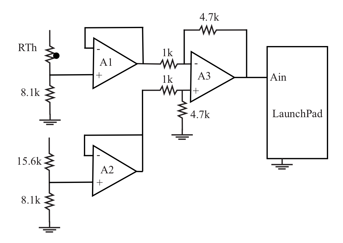
We end up with \(V_{out} = 4.7 \times (V_{in} - 1.13)\), which we can implement with a difference amplifier. Because the thermistor and reference resistor are around 10 \(k\Omega\), we will need input resistors for the difference amplifier that are much larger, in the \(M\Omega\) range, or we will need to use an isolation amplifier (a unity-gain buffer) between the resistor chain and the difference amplifier. Here is a possible circuit.
Amplifier A1, connected as a unity-gain buffer, isolates the voltage from the resistor chain with the thermistor from the input impedance of the difference amplifier, A3. Similarly, A2 isolates the offset voltage of 1.13 V generated by the fixed resistor chain. Amplifier A3 with its four associated resistors is a gain-of–4.7 difference amplifier whose output is given by \(Vout = 4.7 \times (V_{in+} - V_{in-})\). Its output then goes directly into the computer’s analog input.
Now if we sit and read the analog input then we will get a number that is (roughly) proportional to temperature. In practice, unless you are very careful, very lucky, and live in the middle of some kind of desert, there will be quite a lot of noise on the input. Here are some numbers read from such a system at a rate of 100 samples per second.
As you see, there is a lot of variation from one value to the next. We want to see underlying slow changes in the average value despite the noise. There are two ways to approach this.
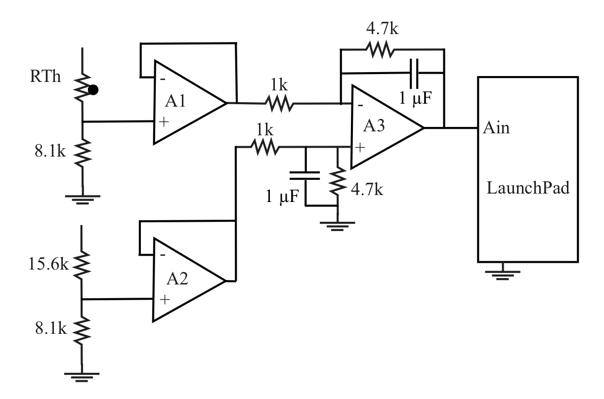
First we can lower the bandwidth of the amplifier so that the high frequency noise is not amplified along with the very low frequency signal. We can do this by putting capacitors across the two 10k resistors. This will create a single-section low-pass filter with cut-off frequency at the usual value. With a 4.7k resistor and a 1 μF capacitor (about the largest practical) we would remove noise above 35 Hz.
Second, we can do the averaging in software. We only care about low frequency information so we only need about 1 sample per second. If we did that literally then we would see all the noise. However, we could also take 100 samples per second and then average them and use the average as our 1 sample per second measurement. This gives us stronger smoothing than the 16 Hz cut-off of the first solution. It is really easy.