Physics 195 Spring 2010 Some Notes on Complex Numbers

This is also available as a PDF here.

Introduction

A little research into the history of complex numbers reveals that, for the first hundred years or so after their introduction, the mathematical community was exactly as fond of complex numbers as most of you are. The rest of the world learned to get along with them in the end so I am sure that you will too but I though it might help if I took a little look at why they are so useful and remind¹ you of some of their properties.

A little basic trigonometry.

I begin by reminding you of a few simple bits of basic trigonometry, to lull you into a false sense of security. You almost certainly met the basic trig functions, sine, cosine, and tangent, in the context of a simple right triangle.²

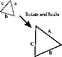
We start from the idea of similar triangles. Two triangles are similar if we can map one onto the other by uniform scaling and rotation. This means that the sides of one triangle a, b, c make the same ratios to each other as the corresponding sides of any other similar triangle, A, B, C. That is

= , = , = , and so on.

This means that these ratios are somehow determined by the angles of the triangles and not by its size. If we then take the right triangle o, a, h we can define the ratios as functions of the lower left angle, θ, thus

sine(θ) = , cosine(θ) = , and tangent(θ) = ,

which we usually abbreviate sinθ,cosθ,tanθ.

We can find the values of a small number of ratios by simple geometry.

For example, a 45^∘ triangle is isoceles so that o = a and h = = a. This means that sin45^∘ = cos45^∘ = = .

Similarly, an equilateral triangle, with all its included angles θ = 60^∘, can be cut in half by a line from one vertex to the middle of the opposite side leaving two 30^∘,60^∘,90^∘ triangles. Now the hypotenuse, h, of one of these triangles must be twice as long as the bisected side, a, so that the third side, the cut side, must have length o = = = = a. Thus the ratios are sin60^∘ = = = , cosθ = = = , and tan60^∘ = = = .

Since we know that the sum of the angles of a trangle is 180^∘ we can deduce that sinθ = cos(90^∘-θ) and cosθ = sin(90^∘-θ) so that sin30^∘ = cos60^∘ = and cos30^∘ = sin60^∘ = giving us tan30^∘ = .

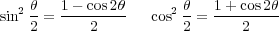
There are a few others we can do this way, but not many. More are available by playing with the double and half angle formulae,

and the sum and difference formulae

Even with these there are practical limits to the anlges whose trig. functions we can find. To complete our understanding we need a more general way to find the values and, while we are at it, to generalize the relations to angles beyond 90^∘, the limit for simple right triangles. This takes us off into the realm of calculus. Once there we will find that the degree is an extremely arbitrary way to measure angle and that the natural unit of measure is the radian defined by the relation between the radius of a circle, r, and the arc traced out by the radius when it moves through an angle θ, a length s. We define the angle to be

so that a complete circle corrseponds to an angle of 2π radians. This has a particularly nice effect for rather small angles when we can treat the arc as being essentially the same length as the chord. In that case we find that as θ → 0 then tanθ → θ, sinθ → θ, cosθ → 1. We call these small angle approximations.

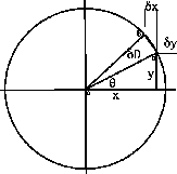
If we take our right triangle and, keeping the length of the hypotenuse constant, vary the angle θ, then the apex of the triangle traces out the arc of a circle. This idea allows us to generalize to angles beyond 90^∘ and it also allows us to study how the trig. functions vary as the angle varies. It allows us to find their derivatives. Lets look at the triangle in the figure formed by sides x, y, and the hypotenuse, oa, of length r. It has included angle θ and we have

Consider a small change δθ in the base angle, a change that is so small that we can treat the arc length ab as being equal to the chord distance and the angle between ab and the original hypotenuse, oa, as 90^∘. The new triangle will have sides of length x + δx, y + δy, and r and an included angle of θ + δθ. Using the sum of angles formulae and the small angle approximations, we find

and

These allow us to find the derivatives from their definitions

That gives us a pair of coupled differential equations for sinθ and cosθ that we can solve in the standard way by differentiating one of the equations and substituting in the other, thus

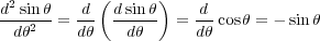
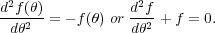
and similarly for cos. Thus sine and cosine are the two independent solutions of the second order differential equation

2-D Plane Geometry

The idea of an imaginary number, a number whose square was negative, began as trick to solve the problem of finding the roots of certain cubic equations. As the name implies, such a number made mathematicians quite uncomfortable. The general acceptance of complex numbers began with the realization that they provide a rather natural algebraic description of much of 2-D plane geometry.

In order to uniquely describe a single point in a 2-D plane you need two coordinates. It had long been known that the description of the plane in terms of coordinates had its simplest, most natural, form if the two coordinates were measured along two mutually perpendicular axes, generally called x and y. You are all familiar with one algebra that results from this practice, the algebra of 2-D vectors. There, we use an external book-keeping mechanism to keep the two coordinates separate, either in columns of numbers, comma separated pairs of numbers, or through the , unit vectors. Complex numbers provide a slightly different method.

The complex method (classically called the Argand Diagram after one of its proponents) takes note of the fact that multiplying a coordinate by -1 rotates the point through 180^∘ about the origin, taking x →-x and y →-y. It then imagines the existence of an operator that rotates you through an anti-clockwise angle of 90^∘ about the origin, taking a point on the x axis to one on the y axis. Let’s call that operation “multiplication by i” and figure out the properties of i, a new kind of number.

1) A point lying a distance d along the horizontal axis can be transformed into a point lying the same distance along the y axis by computing either id or di. So the number representing a point on the y axis can be written iy.

2) Two successive 90^∘ rotations should make up a 180^∘ rotation. Thus, rotating a point lying a distance d up the y axis will be rotated onto the -x axis by the same 90^∘ rotation so that iid →-d.

3) This must be a new kind of number. First because there is no ordinary number whose square is -1. Second because it requires a modification of one of the standard rules of algebra. If a and b are real numbers then × = but this new number gives × = - with an extra minus sign.

4) Using this new kind of number we can map all the points of the 2-D plane to unique points of the form x + iy where x is the perpendicular distance between the point and the y axis and y the perpendicular distance to the x axis. This has the simple interpretation of x in the real direction plus y in the direction at 90^∘ to the real axis. We call such a number a complex number.

5) Addition and subtraction of complex numbers correspond exactly to addition and subtraction of 2-D vectors according to the triangle rules since the real and imaginary parts are not mixed by the operation.

Euler’s Theorem

Consider a point on the unit circle. In complex notation this must be given by a pair of functions x(θ) and y(θ) so that we have r(θ) = x(θ) + iy(θ) where θ is the angle between the x axis and radius to the point. Now let us use the geometric properties of the circle to find differential equations for the functions x(θ) and y(θ).

We start by noting that the constancy of the circle’s radius gives us x(θ)² + y(θ)² = 1.

Now make a differential change dθ in the angle, rotating the point a small distance round the circle in the clockwise direction. We have seen that this defines a difference vector, dr(θ), that is rotated through 90^∘ from the original vector and that has length dθ so that = + i is a unit vector rotated through 90^∘ from the original vector.

Now we have introduced i as a symbol for the operation of rotation through 90^∘ so that we must have

This can thus be viewed either as a single differential equation for the complex valued function r(θ) or a as a pair of coupled differential equations for the two real valued fuctionsx(θ) and y(θ).

If we take the first view then the system is very easy to solve because we know that the solution to a differential equation of the form = aξ is f(ξ) = Ae^aξ where A is a constant of integration. Thus we must have r(θ) = Ae^iθ and the initial condition r(0) = 1 gives us A = 1 so that r(θ) = e^iθ. This function is defined through its power series in the usual fashion, though there is a little extra thought needed to prove that the series converges for all finite values of θ.

If we take the second view of the sytem then we have the coupled equations = -y(θ) (from the real parts) and = x(θ) (from the imaginary parts) which we recognise form above as the differential equation of simple harmonic motion. The solutions are y(θ) = Asin(θ) + B cos(θ) and we can use the boundary conditions x(0) = 1 and y(0) = 0 to find that x(θ) = cos(θ) and y(θ) = sin(θ).

Now we can compare our solutions to find that r(θ) = e^iθ = x(θ) + iy(θ) = cos(θ) + isin(θ) and we have deduced Euler’s equation from the geometry of the situation!